BDS 761: Data Science and Machine Learning I

Topic 7: Graph and Network Methods
I. Introduction to Graphs
Motivation
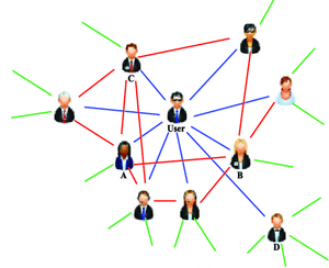
Graphs & Networks are used to describe relationship structures.
Example: Social network - a description of the relationships between people
Disease factor causation?
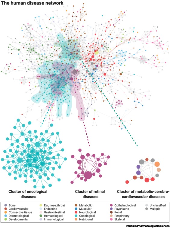
Nogales, Cristian, et al. "Network pharmacology: curing causal mechanisms instead of treating symptoms." Trends in pharmacological sciences 43.2 (2022): 136-150.
Brain activity
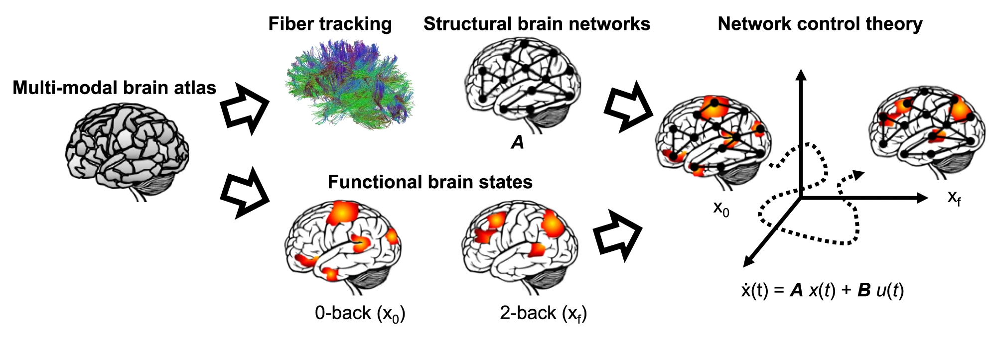
Braun, Urs, et al. "Brain network dynamics during working memory are modulated by dopamine and diminished in schizophrenia." Nature communications 12.1 (2021): 3478.
Graph Definition
$$G = (V,E)$$
- A set of Nodes $V=\{v_1, ..., v_n\}$
- A set of Edges $E = \{e_1, ..., e_m\}, e_i \in V\times V $ - either binary (there or not there) or weighted, between pairs of nodes
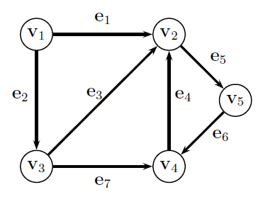
Adjacency Matrix
an $n\times n$ matrix $\mathbf A$ where...
- $A_{i,j}=+1$ if there is an edge from nodes $i$ to $j$
- $A_{j,i}=+1$ if there is an edge from nodes $j$ to $i$

$$\mathbf A = \begin{bmatrix} 0 & 1 & 1 & 0 & 0\\ 1 & 0 & 1 & 1 & 1\\ 1 & 1 & 0 & 1 & 0\\ 0 & 1 & 1 & 0 & 1\\ 0 & 1 & 0 & 1 & 0 \end{bmatrix} $$
Adjacency matrix interpretation
Diffusion operator - applying $\mathbf A$ to vector of values at nodes results in values at neighboring nodes.
Eigenvector intuition - consider what it means, therefore, if $\mathbf A \mathbf x = \lambda \mathbf x$
Degree
Node Degree - $d(v_i)$ number of edges entering or leaving node $v_i$ = In_degree + out_degree
Degree Matrix - diagonal matrix of node degrees
$$\mathbf D = \begin{bmatrix} d_{1} & 0 & 0 & 0 & 0\\ 0 & d_{2} & 0 & 0 & 0\\ 0 & 0 & d_{3} & 0 & 0\\ 0 & 0 & 0 & d_{4} & 0\\ 0 & 0 & 0 & 0 & d_{5} \end{bmatrix} = \begin{bmatrix} 2 & 0 & 0 & 0 & 0\\ 0 & 4 & 0 & 0 & 0\\ 0 & 0 & 3 & 0 & 0\\ 0 & 0 & 0 & 3 & 0\\ 0 & 0 & 0 & 0 & 2 \end{bmatrix} $$
Consider ohw to compute this from adjacency matrix
Adjacency Matrix - Variants
- Signed
- Directed
- Weighted (often called $\mathbf W$)
Consider what each can be used to represent.
Also can have any combination of these properties.
Network methods overwhelmingly focus on unsigned, undirected, binary case. Weighted version also common.
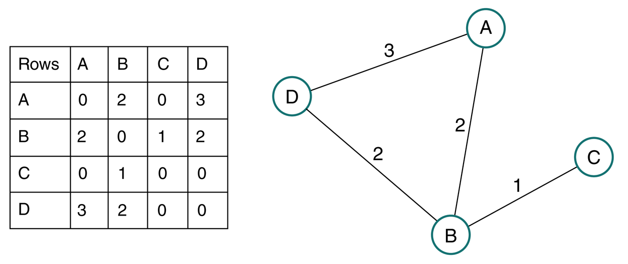
Weighted graph
Generally define weight matrix $\mathbf W$ as weighted analog to adjacency matrix, since also can define a binary adjacency matrix for same graph.
Degree of node in weighted graph is sum of weights of edges connecting node
Degree vector $\mathbf d = \mathbf W \mathbf 1$
Degree matrix $\mathbf D = \text{diag}(\mathbf d)$
import matplotlib.pyplot as plt
import networkx as nx
import numpy as np

A = np.random.rand(5,5)
A = (A>0.5).astype(int)
print(A)
G = nx.from_numpy_matrix(np.matrix(A), create_using=nx.DiGraph)
layout = nx.spring_layout(G)
nx.draw(G, layout)
#nx.draw_networkx_edge_labels(G, pos=layout)
nx.draw_networkx_labels(G, pos=layout)
plt.show();
[[1 0 0 0 1]
 [0 1 0 1 1]
 [0 0 0 0 1]
 [1 1 1 0 1]
 [0 1 0 1 0]]
Creating Networks from data
For a set of variables $\{x_1, ..., x_m\}$
We have a vector of samples of each of the random variables $\{\mathbf x_1, ..., \mathbf x_m\}$
We also like to create a matrix of data $\mathbf X$ from the vectors, where rows are samples and columns are features
Defining edges
- truncated distance: $\Vert \mathbf x_i - \mathbf x_j\Vert < d_{c}$
- similarity: $\exp\left( -\frac{1}{2\sigma^2}\Vert \mathbf x_i - \mathbf x_j\Vert\right)$
Using Covariance matrix as a Weighted adjacency matrix
Consider the choice $\mathbf W = \mathbf C \propto \mathbf X \mathbf X^T$
What is $W_{ij}$ in terms of data samples?
Note relationship to distance
II. Gaussian Graphical Models
Review: Normal a.k.a. Gaussian Distribution $X \sim N(\mu, \sigma) = G(\mu, \sigma)$
$$ f(x) = \frac{1}{\sigma \sqrt{2 \pi}} exp \left(- \frac{(x - \mu)^2}{2 \sigma^2} \right) \text{, for } x \in R $$

import numpy as np
from matplotlib import pyplot as plt

def univariate_normal(x, mean, var):
    return ((1. / np.sqrt(2 * np.pi * var)) * np.exp(-(x - mean)**2 / (2 * var)))

x = np.linspace(-5,5,1000)
plt.plot(x,univariate_normal(x,1,2));
plt.show()
Review: Joint Distributions

Each "sample" as a list of features, which we model as a vector of random variables, $ \mathbf x = \begin{pmatrix} Diameter \\ Thickness \end{pmatrix}
\begin{pmatrix} x_1 \\ \vdots \\ x_n \\ \end{pmatrix} $
Each point in the distribution is simultanous probability of all the features taking the particular vector of numbers at the point.
Multivariate Data - describing relationships
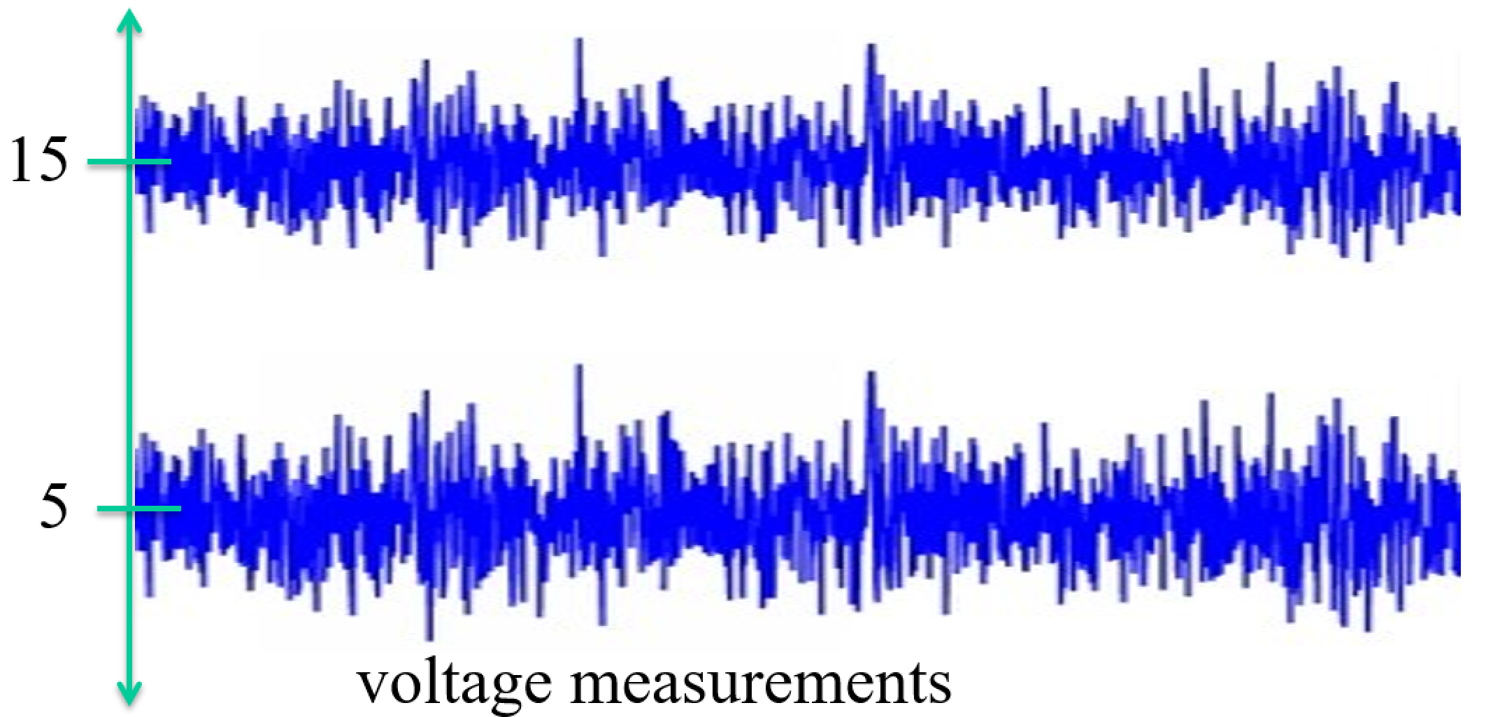
"Multivariate" dataset ~ a matrix with samples for rows and features for columns. Each column (a.k.a. feature) is also known as a variable.
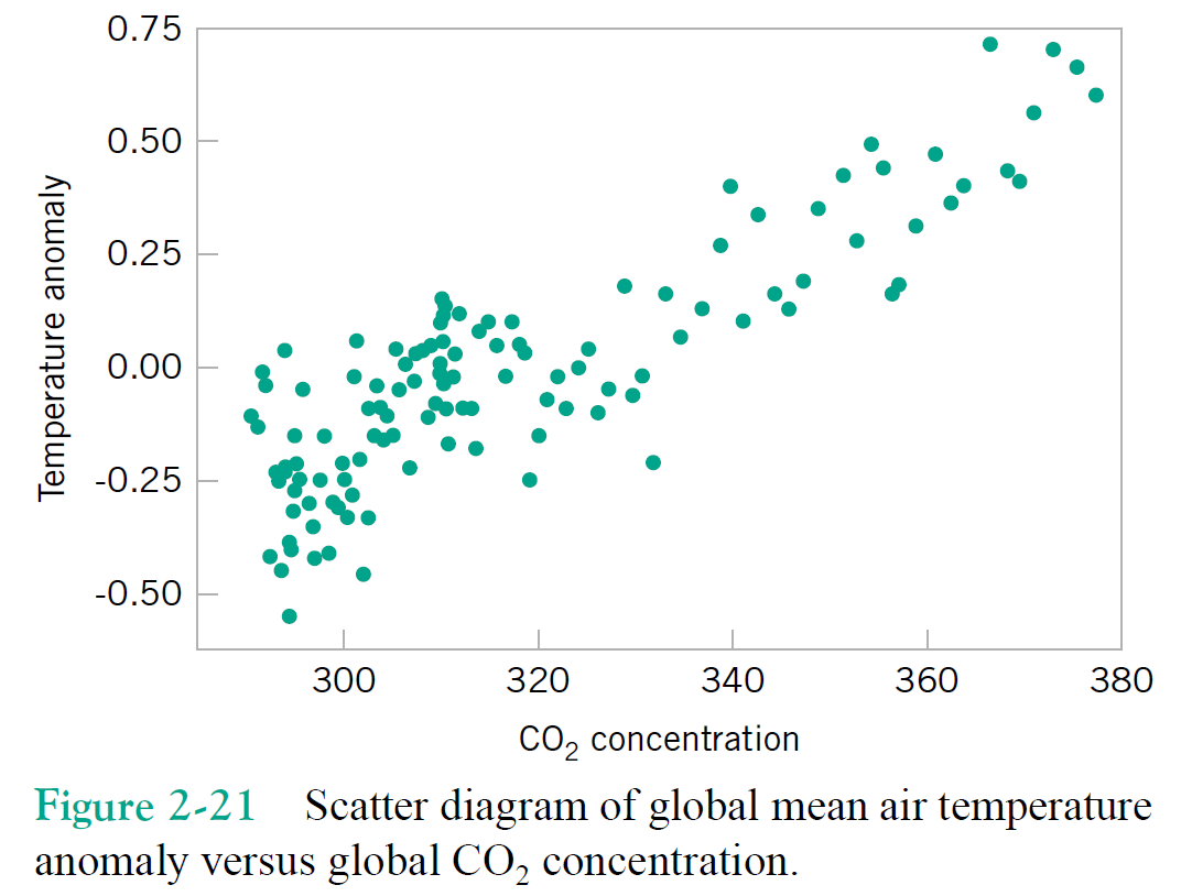
Just focusing on two variables for the moment, say column1 = $x$, and column2 = $y$.
Correlation(s)
\begin{align} \text{Variance} &= s^2 = \frac{\sum_{i=1}^n (x_i - \bar{x})^2}{n - 1} = \frac{\sum_{i=1}^n x_i^2 - \frac{1}{n}(\sum_{i=1}^n x_i)^2}{n - 1} \\ \text{Standard deviation} &= \sqrt{\text{Variance}} \end{align}
\begin{align} \text{Correlation Coefficient} &= r = \frac{ \sum_{i=1}^n (x_i - \bar{x})(y_i - \bar{y})}{\sqrt{\sum_{i=1}^n(x_i - \bar{x})^2}\sqrt{\sum_{i=1}^n(y_i - \bar{y})^2}} = \frac{S_{xy}}{\sqrt{S_{xx} S_{yy}}} \\ %\text{''Corrected Correlation''} % &= S_{xy} = \sum_{i=1}^n (x_i - \bar{x})(y_i - \bar{y}) % = \sum_{i=1}^n x_i y_i - \frac{1}{n}(\sum_{i=1}^n x_i)(\sum_{i=1}^n y_i) \\ \text{Covariance} &= S_{xy} = \frac{1}{n-1}\sum_{i=1}^n (x_i - \bar{x})(y_i - \bar{y}) % = \sum_{i=1}^n x_i y_i - \frac{1}{n}(\sum_{i=1}^n x_i)(\sum_{i=1}^n y_i) \end{align}
Look kind of familiar? Relate to variance. Note $"Cov(x,x)" = S_{xx}= \sigma_x^2$.
Exercises
\begin{align} \text{Correlation Coefficient} &= r = \frac{ \sum_{i=1}^n (x_i - \bar{x})(y_i - \bar{y})}{\sqrt{\sum_{i=1}^n(x_i - \bar{x})^2}\sqrt{\sum_{i=1}^n(x_i - \bar{x})^2}} = \frac{S_{xy}}{\sqrt{S_{xx} S_{yy}}} \end{align}

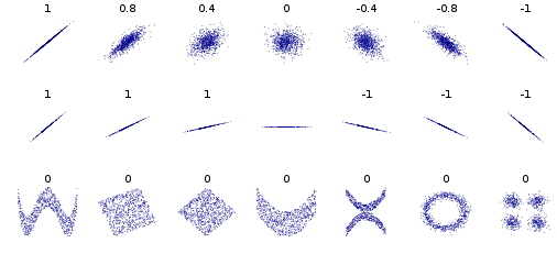
Roughly what are the correlation coefficients here?
Correlation Qualitative Behavior
- What does magnitude tell you about the relationship?
- What does sign tell you about the relationship?
- Would you expect the Covariance to be similar?
Multivariate Gaussian (for $n$ dimensions)
$$ f(\mathbf x) = \frac{1}{ \sqrt{2 \pi^n |\boldsymbol\Sigma|}} \exp \left(- \frac{1}{2} (\mathbf x - \boldsymbol \mu)^T \boldsymbol\Sigma^{-1} (\mathbf x - \boldsymbol \mu) \right) \text{, for } \mathbf x \in R^n $$
- Mean vector as centroid of distribution
- Covariance matrix describes spread - correlations between variables $\Sigma_{ij} = S_{\mathbf x_i \mathbf x_j}$
\begin{align} \text{Correlation Coefficient} &= r = \frac{ \sum_{i=1}^n (x_i - \bar{x})(y_i - \bar{y})}{\sqrt{\sum_{i=1}^n(x_i - \bar{x})^2}\sqrt{\sum_{i=1}^n(y_i - \bar{y})^2}} = \frac{S_{xy}}{\sqrt{S_{xx} S_{yy}}} \\ %\text{''Corrected Correlation''} % &= S_{xy} = \sum_{i=1}^n (x_i - \bar{x})(y_i - \bar{y}) % = \sum_{i=1}^n x_i y_i - \frac{1}{n}(\sum_{i=1}^n x_i)(\sum_{i=1}^n y_i) \\ \text{Covariance} &= S_{xy} = \frac{1}{n-1}\sum_{i=1}^n (x_i - \bar{x})(y_i - \bar{y}) % = \sum_{i=1}^n x_i y_i - \frac{1}{n}(\sum_{i=1}^n x_i)(\sum_{i=1}^n y_i) \end{align}
...Terminology note...
In general terms, covariance is a kind of metric for correlation.
Formal definition of correlation (i.e. Pearson) differs from covariance only in scaling, so that it ranges between $\pm 1$ rather than some max and min.
I will tend to use them interchangeably, where correlation means the more intuitive concept and covariance the formal matrix we compute (or its elements).
def multivariate_normal(x, n, mean, cov):
    return (1./(np.sqrt((2*np.pi)**n * np.linalg.det(cov))) * np.exp(-1/2*(x - mean).T@np.linalg.inv(cov)@(x - mean)))


mean = np.array([35,70])
cov = 100*np.array([[1,.5],[.5,1]])
pic = np.zeros((100,100))
for x1 in np.arange(0,100):
    for x2 in np.arange(0,100):
        x = [x1,x2]
        pic[x1,x2] = multivariate_normal(x, 2, mean, cov)

plt.contour(pic);
cov
array([[100.,  50.],
       [ 50., 100.]])
np.linalg.inv(cov)
array([[ 0.01333333, -0.00666667],
       [-0.00666667,  0.01333333]])
Exercise: independence of random variables
$$P(x_1,x_2) = P(x_1)P(x_2)$$
What does the mean for a multivariate Gaussian distribution?
Precision and Precision Matrix
The Precision of a variable is commonly (though not always) defined as the inverse of the variance. $p = \sigma^{-2}$.
Higher spread means higher variance and hence lower precision.
The Precision Matrix is the inverse of the Covariance matrix. $\mathbf P = \boldsymbol\Sigma^{-1}$.
This matrix is used in the multivariate Gaussian.
Gaussian graphical models
Recall from Bayesian networks that correlation does not imply causation.
It is much more interesting to describe the conditional correlation (a.k.a. partial correlation) between variables, rather than simply the correlation.
If conditional correlation is zero, the variables are conditionally independent.
Amazingly, partial correlations are closely-related to the inverse of the covariance matrix, $\mathbf\Sigma^{-1}$, also called the precision matrix.
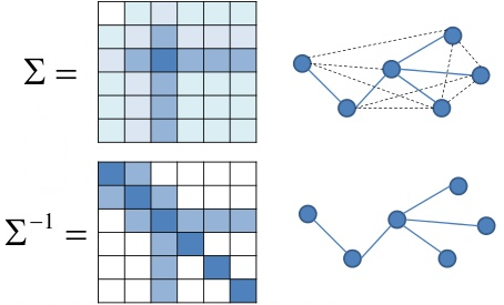
Also known as Gauss Markov Random Fields
Partial correlation and precision matrix
The partial correlation between a pair of variables, conditioned on all the rest, is related (within a scalar) to the $(i,j)$th element of the precision matrix.
\begin{align} \rho_{i,j} = -\frac{\sigma^{i,j}}{\sqrt{\sigma^{i,i}\sigma^{j,j}}} \end{align}
Hence a pair of variables $x_i$ and $x_j$ are conditionally independent if $\sigma^{(i,j)}=0$.
A zero implies conditional independence for a variety of non-Gaussian cases also
Recap
We start by considering a set of random variables $\{x_1, ..., x_m\}$
In practice we will use a vector of samples of each of the random variables $\{\mathbf x_1, ..., \mathbf x_m\}$
We like to create a matrix of data $\mathbf X$ from the vectors, where rows are samples and columns are features
If we subtract the means from each row, we can compute a sample covariance matrix $\mathbf C = \frac{1}{N-1} \mathbf X \mathbf X^T$. (often we ignore the scalar term).
If $\mathbf C$ is invertible, we can estimate the precision matrix $P = \mathbf C^{-1}$.
Nonzero elements of the precision matrix $\sigma^{i,j}$ give edges in the graphical model.
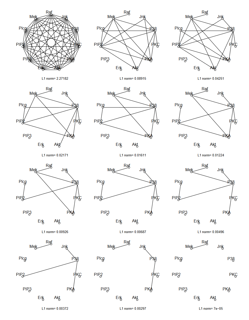
However generally hard zeros don't occur in real data calculations. Instead of thresholding the covariance matrix to make a sparse network, we can threshold the precision matrix.
Graphical Lasso
Instead of thresholding the precision matrix values, we can seek a sparse (approximate) inverse to $\mathbf C$
\begin{align} f(\mathbf x) &= \frac{1}{ \sqrt{2 \pi^n |\boldsymbol\Sigma|}} \exp \left(- \frac{1}{2} (\mathbf x - \boldsymbol \mu)^T \boldsymbol\Sigma^{-1} (\mathbf x - \boldsymbol \mu) \right) \\ &= \frac{\sqrt{|\boldsymbol\Omega|}}{ \sqrt{2 \pi^n }} \exp \left(- \frac{1}{2} (\mathbf x - \boldsymbol \mu)^T \boldsymbol\Omega (\mathbf x - \boldsymbol \mu) \right) \\ &= \frac{\sqrt{|\boldsymbol\Omega|}}{ \sqrt{2 \pi^n }} \exp \left(- \frac{1}{2} \text{trace}(\mathbf S \boldsymbol\Omega)\right) \end{align}
Where now $\mathbf S$ is the sample covariance matrix and $\boldsymbol\Omega$ is the precision matrix (whice we view as approximations to $\boldsymbol\Sigma$ and $\boldsymbol\Sigma^{-1}$, respectively)
Graphical Lasso - continued
Now we view $\boldsymbol\Omega$ as the random variable and $\mathbf S$ as the data, so we have the likelihood
\begin{align} P(\mathbf S|\boldsymbol\Omega) = f(\mathbf x) = &= \frac{\sqrt{|\boldsymbol\Omega|}}{ \sqrt{2 \pi^n }} \exp \left(- \frac{1}{2} \text{trace}(\mathbf S \boldsymbol\Omega)\right) \end{align}
We wish to compute a sparse estimate for $\boldsymbol\Omega$ so use the prior $p(\lambda\boldsymbol\Omega) \propto \exp(\Vert\boldsymbol\Omega\Vert_1)$ and Bayes law to compute
\begin{align} P(\boldsymbol\Omega |\mathbf S) &= \frac{P(\mathbf S|\boldsymbol\Omega) P(\boldsymbol\Omega)}{P(\mathbf S)} \end{align}
The maximum likelihood solution, subject to a constraint that $\boldsymbol\Omega$ has non-negative eigenvalues (hence is a legitimate precision matrix):
\begin{align} \arg\max_{\boldsymbol\Omega \succeq 0} P(\boldsymbol\Omega |\mathbf S) &= \arg\max_{\boldsymbol\Omega \succeq 0} \frac{P(\mathbf S|\boldsymbol\Omega) P(\boldsymbol\Omega)}{P(\mathbf S)} \\ &= \arg\max_{\boldsymbol\Omega \succeq 0} P(\mathbf S|\boldsymbol\Omega) P(\boldsymbol\Omega) \\ &= \arg\max_{\boldsymbol\Omega \succeq 0} \log\{ P(\mathbf S|\boldsymbol\Omega) P(\boldsymbol\Omega) \} \\ &= \arg\max_{\boldsymbol\Omega \succeq 0} \{ \log|\boldsymbol\Omega| - \text{trace}(\mathbf S \boldsymbol\Omega) - \lambda\Vert\boldsymbol\Omega\Vert_1 \}\\ \end{align}
Long story short
compute covariance matrix of data, $\mathbf S$
Choose hyperparameter $\lambda$ to tune sparse prior (higher=sparser) and compute optimal $\arg\max_{\boldsymbol\Omega \succeq 0} \{ \log|\boldsymbol\Omega| - \text{trace}(\mathbf S \boldsymbol\Omega) - \lambda\Vert\boldsymbol\Omega\Vert_1 \}$
Form graph given that nonzero elements of $\boldsymbol\Omega$ mean conditional independence.
Example
Friedman and Hastie and Tibshirani "Sparse inverse covariance estimation with the graphical lasso", Biostatistics 2008
Regression approach: Neighborhood estimation problem
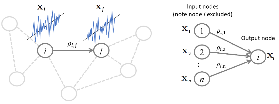
Regression problem for relating all other variables to a given variable
\begin{align} x_i = \sum_{k \neq i} \beta_{i,k} x_k + \epsilon_i, \end{align}
Partial correlation, precision matrix, and regression coefficients
The partial correlation between a pair of variables, conditioned on all the rest, is related by a scalar to the $(i,j)$th element of the precision matrix.
A pair of variables $x_i$ and $x_j$ are conditionally independent if the linear regression coefficient $\beta_{i,j}=0$.
\begin{align} \rho_{i,j} = -\frac{\sigma^{i,j}}{\sqrt{\sigma^{i,i}\sigma^{j,j}}} &= -\beta_{i,j} \sqrt{\frac{\sigma^{i,i}}{\sigma^{j,j}}}, \end{align}
Regression-based methods for estimating edges
Loop over all nodes and regress versus all others using your favorite regression method
can impose sparsity and other priors, can use efficient greedy methods
Linear Algebra view of Regression
The regression problem relating random variables $x_i$ is
\begin{align} x_i = \sum_{k \neq i} \beta_{i,k} x_k + \epsilon_i, \end{align}
We use a vector of samples of each of the random variables $\{\mathbf x_1, ..., \mathbf x_m\}$
Then each neighborhood regression problem is
\begin{align} \mathbf x_i = \sum_{k \neq i} \mathbf x_k \beta_{i,k} + \boldsymbol\epsilon_i, \end{align}
If we don't exclude the $i$th node from the sum (effectively allowing self-loops) we can write
\begin{align} \mathbf x_i = \mathbf X^T \boldsymbol\beta_{i} + \boldsymbol\epsilon_i, \end{align}
Using matrix of data $\mathbf X$ where rows are samples $\mathbf x_i^T$ and columns are features. And $\boldsymbol\beta_{i}$ is the vector of coefficients $\beta_{i,k}$ relating the other nodes to the $i$th node.
Exercises
Draw a little network and relate it to $\mathbf X$ and $\boldsymbol\beta_{i}$
Combine all the regression problems for all nodes into a single equation
Least squares solution
Suppose our dataset matrix $\mathbf X$ is not invertible.
The least squares solution to $\mathbf X^T \mathbf B = \mathbf X^T$ is $\mathbf B = (\mathbf X^T)^\dagger \mathbf X^T$ using the pseudoinverse
If the SVD of $\mathbf X^T$ is $\mathbf U \mathbf S \mathbf V^T$ then we can write the SVD of $(\mathbf X^T)^\dagger$ as $\mathbf V \mathbf S\dagger \mathbf U^T$, where $S\dagger$ is a rectangular diagonal matrix with the inverses of the nonzero singular values of $\mathbf X^T$ on the diagonal (and zero otherwise).
Multiplying this out we get
\begin{align} \mathbf B &= (\mathbf X^T)^\dagger \mathbf X^T \\ &= (\mathbf V \mathbf S^\dagger \mathbf U^T)(\mathbf U \mathbf S \mathbf V^T) \\ &= \mathbf U_r \mathbf U_r^T \end{align}
where $\mathbf U_r$ is the matrix of singular vectors for the $r$ nonzero singular values of $\mathbf X^T$.
Regression as Embedding
Consider the distances between rows of the matrix of regression coefficients $\mathbf B = \mathbf U_r \mathbf U_r^T $
\begin{align} d(i,j) &= \Vert \mathbf b^{(i)} - \mathbf b^{(j)} \Vert \\ &= \Vert \mathbf u_r^{(i)} \mathbf U_r^T - \mathbf u_r^{(j)} \mathbf U_r^T \Vert \\ &= \Vert (\mathbf u_r^{(i)} - \mathbf u_r^{(j)}) \mathbf U_r^T \Vert \\ &= \Vert \mathbf u_r^{(i)} - \mathbf u_r^{(j)} \Vert \\ \end{align} Where we use the fact that an orthogonal transformation does not change the distance (with a $\ell_2$-norm)
So the regression coefficient matrix is equivalent to a particular case of spectral embedding of the data
III. Spectral Clustering
Famous Matrices: Diagonal matrix
$$\mathbf D = \begin{bmatrix} D_{1,1} & 0 & 0\\ 0 & D_{2,2} & 0 \\ 0 & 0 & D_{3,3}\\ \end{bmatrix}$$
Consider what it implies for a linear system with a diagonal matrix.
Can completely describe with a vector $\mathbf d$ with $d_i = D_{i,i}$
Hence we write "$\mathbf D = \text{diag}(\mathbf d)$" and "$\mathbf d = \text{diag}(\mathbf D)$"
Relate to Hadamard product of vectors $\mathbf D \mathbf v = \mathbf d \odot \mathbf v$.
Famous Matrices: Diagonal matrix - Applications
Consider product $\mathbf D \mathbf v$
Consider products $\mathbf D \mathbf A$ and $\mathbf A \mathbf D$
Consider norm $\Vert \mathbf D \mathbf v \Vert_2$
Consider $\mathbf D_1 \mathbf D_2$
Consider power $\mathbf D^n$
Consider inverse of diagonal matrix $\bf D$
Solve linear system $\mathbf A \mathbf x = \mathbf b$ when $\mathbf A$ is diagonal.
Famous Matrices: Orthogonal matrix
Square marix where columns are orthogonal, i.e. $\mathbf a_i^T \mathbf a_j = 0$ when $i \ne j$
Orthonormal matrix $\rightarrow$ also have $\mathbf a_i^T \mathbf a_i = 1$
Famous Matrices: Orthogonal matrix - Applications
Geometrically, orthonormal matrices implement rotations.
Very easy inverse
Solve linear system $\mathbf U \mathbf x = \mathbf b$ for $\mathbf x$ when $\mathbf U$ is orthonormal.
Solve matrix system $\mathbf U \mathbf A = \mathbf V$ for $\mathbf A$ when $\mathbf U$ is orthonormal.
Eigendecomposition
Reconsider: $${\bf A}{\bf u} = \lambda {\bf u}$$
IF $\mathbf A$ is $n \times n$ symmetric and real, we can find $n$ eigenvectors $\{ \mathbf u_i \}$ with corresponding real eigenvalues $\lambda_i$, i.e.
$${\bf A}{\bf u_i} = \lambda_i {\bf u_i}$$
If the eigenvalues are distinct, the eigenvalues are orthogonal. Otherwise they may not be orthogonal but are still linearly independent, so we can make an orthogonal basis.
Write this as ${\bf A}{\bf U} = $ ?
Diagonalization
a.k.a. Eigendecomposition
a.k.a. Spectral Decomposition)
$$ {\bf A}{\bf U} = {\bf U} \boldsymbol\Lambda \rightarrow {\bf A} = {\bf U} \boldsymbol\Lambda {\bf U}^{-1} $$
We can also solve for $\boldsymbol\Lambda$ = ?
Famous Matrices: Normal matrix
A real matrix $\bf A$ is a normal matrix if:
$$ \mathbf A \mathbf A^T = \mathbf A^T \mathbf A$$
Note this must be a square matrix due to matrix multiplication rules.
Examples of Normal matrices:
$\mathbf A = \mathbf B \mathbf B^T$ for some $m \times n$ matrix $\bf B$
$\mathbf A = \mathbf B^T \mathbf B$ for some $m \times n$ matrix $\bf B$
Famous Matrices: Normal matrix - value
If a real matrix $\bf A$ is a normal matrix then its eigenvectors are orthonormal.
$$ {\bf A}{\bf U} = {\bf U} \boldsymbol\Lambda \rightarrow ? $$
Graph Laplacians
Unnormalized - binary graphs: $ \mathbf L = \mathbf D - \mathbf A $, weighted graphs: $ \mathbf L = \mathbf D - \mathbf W $
Symmetric: $ \mathbf L_{sym} = \mathbf D^{-\frac{1}{2}} \mathbf L \mathbf D^{-\frac{1}{2}} $
Random walk: $ \mathbf L_{rw} = \mathbf D^{-1} \mathbf L $
Spectral Graph Drawing (a.k.a. Embedding)
The drawing of a graph is a function $\boldsymbol\rho(\cdot)$ which assigns a point in space $\boldsymbol\rho(v_i)$ to each node $v_i$
The matrix $\mathbf R$ of a graph drawing is a $m\times n$ matrix whos $i$th row is $\boldsymbol\rho(v_i)$
Energy of a drawing
View edges as springs and our goal is to make a graph with minimum energy stored in the springs
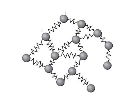
Weight of edge is strength of spring
\begin{align} \varepsilon(R) &= \sum_{\text{edges} \;i\leftrightarrow j} w_{ij} \Vert\boldsymbol\rho(v_i) -\boldsymbol\rho(v_j)\Vert^2 \\ &= \text{trace}(\mathbf R^T \mathbf L \mathbf R) \end{align}
So a high edge weight means the nodes want to be close together
Balanced Orthogonal Drawing
Representation is balanced if $\mathbf 1^T \mathbf R = \mathbf 0^T$ - sum of columns is zero
To prevent trivial solutions (e.g. all nodes placed at the origin) we add the constraint that $\mathbf R$ is an orthogonal matrix, i.e. $\mathbf R^T \mathbf R = \mathbf I$
Minimum Energy Balanced Orthogonal Drawing
For a weighted Graph Laplacian $\mathbf L$
with eigenvalues $0=\lambda_1<\lambda_2\le \lambda_3 \le... \le \lambda_m$
The Minimum Energy Balanced Orthogonal Drawing has energy $\lambda_2+...+\lambda_{n+1}$ (where $n<m$).
The representation $\mathbf R$ consisting of the associated unit eigenvectors $u_2,...,u_{n+1}$ achieves this minimum energy.
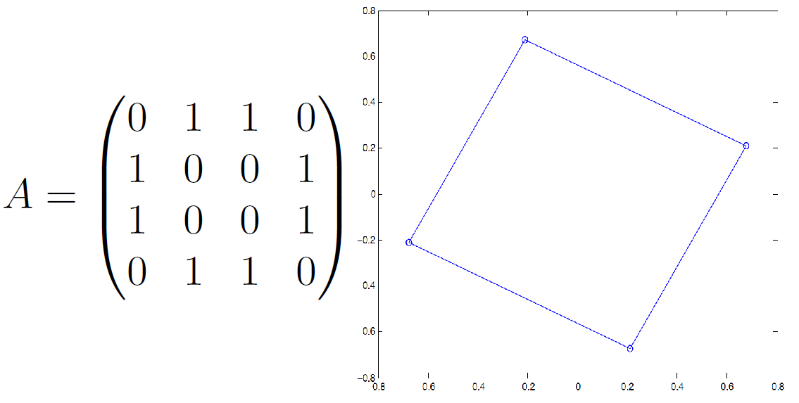
2D Case
- Compute 2nd and 3rd eigenvectors $\mathbf u_2$ and $\mathbf u_3$, i.e. corresponding to two smallest nonzero eigenvalues
- Form $m\times 2$ representation matrix $\mathbf R = (\mathbf u_2, \mathbf u_3)$ with eigenvectors as columns
- Place node $v_i$ at point defined by $i$th row of $\mathbf R$
Example
Network Embedding versus "Data Embedding"
Note when dealing with network methods we have two possible starting points:
- Starting with an already-made network (given an adjacency matrix describing connections between a set of nodes)
- Starting with a dataset (given a matrix of samples versus features), where the first step is to form the network (somehow)
In #2, we start with a set of sample vectors, then compute a bunch of embedded model locations, which might be viewed as new sample vectors (now in a lower number of dimensions).
What are other names used for approach #2?
Graph cut
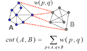
Starting with a graph $G=(V,E)$
We choose a subset of nodes $U \subset V$, where $\bar{U}$ is the set of nodes in $V$ that are not in $U$
$$ \text{cut}(U) \equiv \sum_{v_i\in U, v_j\in \bar{U}} w_{ij} $$
The sum of weights of edges we would cut to remove $U$ from $V$
Multiple cluster version ($K$ = # clusters)
$$ \text{cut}(U_1,...U_K) \equiv \frac{1}{2} \sum_{i} \text{cut}(U_i) $$
Mincut problem
Choose subset $U^*$ that minimizes cut: $$ \arg\min_U \text{cut}(U) $$
- Describe subset(s) with a class vector $\mathbf c$
- For $K=2$, have $c_i\in \{0,1\}$
- For general $K$, have $c_i\in [0,1,...,K]$
For $K=2$ can be solved efficiently, however algorithms which minimize the cut often end up with a trivial solution which chooses a subset consisting of a single node.
This is addressed by changing the problem to make these trivial solutions less likely. For example by weighting the objective by the size of the subset (so smaller subsets are less desirable).
Normalized cut
$$ \text{NCut}(U_1,...,U_K) \equiv \sum_{i} \frac{\text{Cut}(U_i,\bar{U}_i)}{\text{Vol}(U_i)} $$
NP-hard optimization problem: $$ \arg\min_{U_1,...,U_K} \text{NCut}(U_1,...,U_K) $$
Spectral Clustering
Continuous relaxation of class membership. Instead of $c_i\in [0,1,...,K]$, allow continuous values for $c_i$. Then choose class based on nearest integers.
$K=2$ case: Jianbo Shi and Jitendra Malik. "Normalized cuts and image segmentation". Transactions on Pattern Analysis and Machine Intelligence, 22(8):888-905, 2000.
$K>2$ case: Stella X. Yu. "Computational Models of Perceptual Organization". PhD thesis, Carnegie Mellon University, 2003 Dissertation; Stella X. Yu and Jianbo Shi. "Multiclass spectral clustering". In 9th International Conference on Computer Vision, IEEE, 2003.
Spectral Clustering, $K=2$ (Shi and Malik)
- Given an image or image sequence, set up a weighted graph $G = (V,E)$ and set the weight on the edge connecting two nodes to be a measure of the similarity between the two nodes.
- Solve $\mathbf L_{sym}\mathbf x = \lambda \mathbf x$ for eigenvectors with the smallest eigenvalues.
- Use the eigenvector with the second smallest eigenvalue to bipartition the graph.
- Decide if the current partition should be subdivided and recursively repartition the segmented parts if necessary.
Shi and Malik. "Normalized cuts and image segmentation". Transactions on Pattern Analysis and Machine Intelligence, 22(8):888-905, 2000.
Spectral Clustering, $K>2$ (Ng, Jordan, & Weiss)
Given a set of points $S = \{\mathbf s_1, ... , \mathbf s_n\}$ with $\mathbf s_i \in \mathbf R^n$ that we want to cluster into $k$ subsets
- Form the affinity matrix defined by $A_{ij} = \exp(-\frac{1}2\sigma\Vert \mathbf s_i - \mathbf s_j\Vert^2)$ if $i \ne j$ , and $A_{ii} = 0$.
- Define $\mathbf D$ to be the diagonal matrix whose $(i, i)$-element is the sum of $\mathbf A$'s $i$th row, and construct the matrix $\mathbf L = \mathbf D^{-\frac{l}{2}} \mathbf A \mathbf D^{-\frac{l}{2}}$
- Find $\mathbf x_1, \mathbf x_2, ..., \mathbf x_k$ , the $k$ largest eigenvectors of $\mathbf L$ (chosen to be orthogonal to each other in the case of repeated eigenvalues), and form the matrix $\mathbf X = (\mathbf x_1, \mathbf x_2, ..., \mathbf x_k)$ by stacking the eigenvectors in columns.
- Form the matrix $\mathbf Y$ from $\mathbf X$ by renormalizing each of $\mathbf X$'s rows to have unit length (i.e. $Y_{ij} = [\sum_j X_{ij}]^{-\frac{1}{2}} X_{ij}$).
- Treating each row of $\mathbf Y$ as a point in $\mathbf R^k$ , cluster them into $k$ clusters via $K$-means or any other algorithm (that attempts to minimize distortion).
- Finally, assign the original point $\mathbf s_i$ to cluster $j$ if and only if row $i$ of the matrix $\mathbf Y$ was assigned to cluster $j$.
Ng, Jordan, Weiss, "On spectral clustering: Analysis and an algorithm" Advances in neural information processing, 2002.
Eigenvector Variants
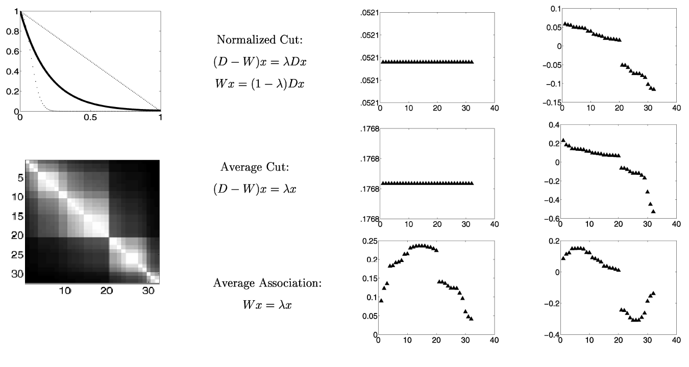
- First one is random walk Laplacian
- Equivalent to using normalized version of weight matrix (unit row sums).
Recap
Assume we start with a dataset and need to form the network to apply spectral graph methods.
Given matrix of data $\mathbf X$ where rows are samples and columns are features
- Form either a weighted adjacency matrix $\mathbf W$ or a binary adjacency matrix $\mathbf A$ via some approach that quantifies similarity between samples.
- Simple approach: take inner product $\mathbf x_i^T \mathbf x_j$ between two samples $\mathbf x_i$ and $\mathbf x_j$ and this as $W_{ij}$ or perhaps use some function of this value such as $|\mathbf x_i^T \mathbf x_j|$.
Compute Laplacian of network such as $\mathbf L = \mathbf D - \mathbf W$ or some other version.
Compute eigenvectors $\mathbf u_1, ..., \mathbf u_k$ for $k$ smallest eigenvalues of $\mathbf L$,
Discard $\mathbf u_1$ and form matrix $\mathbf U$ with $\mathbf u_2, ..., \mathbf u_k$ as columns.
Use rows of $\mathbf U$ as embedded samples.
Cluster these embedded samples to perform partitioning of graph and therefore of original samples.
Caveat Roundup
We also assumed the graph makes a single connected component. If we are automatically generating a big sparse graph from a dataset, this assumption may be violated. In general, for a non-negative weighted graph the first eigenvalue (which takes value 0 and has eigenvector $\mathbf 1$) will have multiplicity equal to the number of connected compoennts. Discard all of these trivial eigenvectors.
For the clustering problem, the choise of clusters $k$ is an open problem (as usual with clustering methods).
We have lots of (vaguely-similar) options for how to compute similarity and therefore the choice of $\mathbf W$ or $\mathbf A$
We have a few (also vaguely-similar) options for choice of Laplacian (unnormalized, symmetric, random walk), and a few more variants depending on less-common kinds of networks (signed, directed)
Don't feel overwhelmed by all these variants. They lead to largely-similar results, though some will work better than others for your problem. For example, thresholding of similarities to use a binary adjacency matrix rather than weighted might make the results a bit more robust vs noise, or less so, depending on the data

